2D Plots
Drawing 2D figures
In this lecture, we will make 2D figures
import numpy as np
import matplotlib.pyplot as plt
from netCDF4 import Dataset, num2date
import matplotlib
# %matplotlib qt
# Figures in a separate window
# %matplotlib inline          # Figures in this browser
Read the temperature data
We are going to read two datasets: one for the mean temperature (absolute.nc) and the other one for the time series of temperature anomaly (HadCRUT.4.6.0.0.median.nc).
f = Dataset('absolute.nc', 'r')
print(f.variables.keys())
T = f.variables['tem'][:]    # monthly data
lon = f.variables['lon'][:]
lat = f.variables['lat'][:]
f.close()
odict_keys(['tem', 'lat', 'lon', 'time'])
f = Dataset('HadCRUT.4.6.0.0.median.nc', 'r')
print(f.variables.keys())
Tanom = f.variables['temperature_anomaly'][:]
time = f.variables['time'][:]
lon = f.variables['longitude'][:]
lat = f.variables['latitude'][:]
# print(f.variables['time'])
f.close()
odict_keys(['latitude', 'longitude', 'time', 'temperature_anomaly', 'field_status'])
The size of Tanom is
T.shape
(12, 36, 72)
Plot temperature 2D plot
Let’s make a plot of T in 1850
T1850 = T[0, :, :] + Tanom[0, :, :] # This is the monthly mean
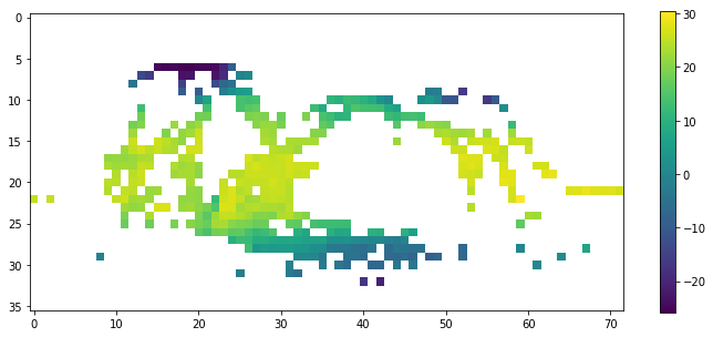
imshow
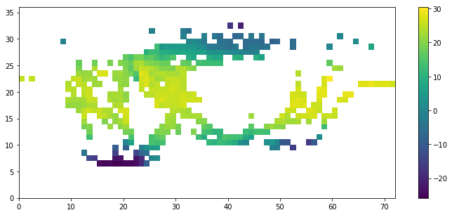
The simplest way to visualize a 2D variable is imshow. This function gives colors to each element of the array without considering grid information. It is fast and a good tool to check the variable.
help(plt.imshow)
Help on function imshow in module matplotlib.pyplot:

imshow(X, cmap=None, norm=None, aspect=None, interpolation=None, alpha=None, vmin=None, vmax=None, origin=None, extent=None, shape=None, filternorm=1, filterrad=4.0, imlim=None, resample=None, url=None, *, data=None, **kwargs)
    Display an image, i.e. data on a 2D regular raster.

    Parameters
    ----------
    X : array-like or PIL image
        The image data. Supported array shapes are:

        - (M, N): an image with scalar data. The data is visualized
          using a colormap.
        - (M, N, 3): an image with RGB values (float or uint8).
        - (M, N, 4): an image with RGBA values (float or uint8), i.e.
          including transparency.

        The first two dimensions (M, N) define the rows and columns of
        the image.

        The RGB(A) values should be in the range [0 .. 1] for floats or
        [0 .. 255] for integers.  Out-of-range values will be clipped to
        these bounds.

    cmap : str or `~matplotlib.colors.Colormap`, optional
        A Colormap instance or registered colormap name. The colormap
        maps scalar data to colors. It is ignored for RGB(A) data.
        Defaults to :rc:`image.cmap`.

    aspect : {'equal', 'auto'} or float, optional
        Controls the aspect ratio of the axes. The aspect is of particular
        relevance for images since it may distort the image, i.e. pixel
        will not be square.

        This parameter is a shortcut for explicitly calling
        `.Axes.set_aspect`. See there for further details.

        - 'equal': Ensures an aspect ratio of 1. Pixels will be square
          (unless pixel sizes are explicitly made non-square in data
          coordinates using *extent*).
        - 'auto': The axes is kept fixed and the aspect is adjusted so
          that the data fit in the axes. In general, this will result in
          non-square pixels.

        If not given, use :rc:`image.aspect` (default: 'equal').

    interpolation : str, optional
        The interpolation method used. If *None*
        :rc:`image.interpolation` is used, which defaults to 'nearest'.

        Supported values are 'none', 'nearest', 'bilinear', 'bicubic',
        'spline16', 'spline36', 'hanning', 'hamming', 'hermite', 'kaiser',
        'quadric', 'catrom', 'gaussian', 'bessel', 'mitchell', 'sinc',
        'lanczos'.

        If *interpolation* is 'none', then no interpolation is performed
        on the Agg, ps and pdf backends. Other backends will fall back to
        'nearest'.

        See
        :doc:`/gallery/images_contours_and_fields/interpolation_methods`
        for an overview of the supported interpolation methods.

        Some interpolation methods require an additional radius parameter,
        which can be set by *filterrad*. Additionally, the antigrain image
        resize filter is controlled by the parameter *filternorm*.

    norm : `~matplotlib.colors.Normalize`, optional
        If scalar data are used, the Normalize instance scales the
        data values to the canonical colormap range [0,1] for mapping
        to colors. By default, the data range is mapped to the
        colorbar range using linear scaling. This parameter is ignored for
        RGB(A) data.

    vmin, vmax : scalar, optional
        When using scalar data and no explicit *norm*, *vmin* and *vmax*
        define the data range that the colormap covers. By default,
        the colormap covers the complete value range of the supplied
        data. *vmin*, *vmax* are ignored if the *norm* parameter is used.

    alpha : scalar, optional
        The alpha blending value, between 0 (transparent) and 1 (opaque).
        This parameter is ignored for RGBA input data.

    origin : {'upper', 'lower'}, optional
        Place the [0,0] index of the array in the upper left or lower left
        corner of the axes. The convention 'upper' is typically used for
        matrices and images.
        If not given, :rc:`image.origin` is used, defaulting to 'upper'.

        Note that the vertical axes points upward for 'lower'
        but downward for 'upper'.

    extent : scalars (left, right, bottom, top), optional
        The bounding box in data coordinates that the image will fill.
        The image is stretched individually along x and y to fill the box.

        The default extent is determined by the following conditions.
        Pixels have unit size in data coordinates. Their centers are on
        integer coordinates, and their center coordinates range from 0 to
        columns-1 horizontally and from 0 to rows-1 vertically.

        Note that the direction of the vertical axis and thus the default
        values for top and bottom depend on *origin*:

        - For ``origin == 'upper'`` the default is
          ``(-0.5, numcols-0.5, numrows-0.5, -0.5)``.
        - For ``origin == 'lower'`` the default is
          ``(-0.5, numcols-0.5, -0.5, numrows-0.5)``.

        See the example :doc:`/tutorials/intermediate/imshow_extent` for a
        more detailed description.

    shape : scalars (columns, rows), optional, default: None
        For raw buffer images.

    filternorm : bool, optional, default: True
        A parameter for the antigrain image resize filter (see the
        antigrain documentation).  If *filternorm* is set, the filter
        normalizes integer values and corrects the rounding errors. It
        doesn't do anything with the source floating point values, it
        corrects only integers according to the rule of 1.0 which means
        that any sum of pixel weights must be equal to 1.0.  So, the
        filter function must produce a graph of the proper shape.

    filterrad : float > 0, optional, default: 4.0
        The filter radius for filters that have a radius parameter, i.e.
        when interpolation is one of: 'sinc', 'lanczos' or 'blackman'.

    resample : bool, optional
        When *True*, use a full resampling method.  When *False*, only
        resample when the output image is larger than the input image.

    url : str, optional
        Set the url of the created `.AxesImage`. See `.Artist.set_url`.

    Returns
    -------
    image : `~matplotlib.image.AxesImage`

    Other Parameters
    ----------------
    **kwargs : `~matplotlib.artist.Artist` properties
        These parameters are passed on to the constructor of the
        `.AxesImage` artist.

    See also
    --------
    matshow : Plot a matrix or an array as an image.

    Notes
    -----
    Unless *extent* is used, pixel centers will be located at integer
    coordinates. In other words: the origin will coincide with the center
    of pixel (0, 0).

    There are two common representations for RGB images with an alpha
    channel:

    -   Straight (unassociated) alpha: R, G, and B channels represent the
        color of the pixel, disregarding its opacity.
    -   Premultiplied (associated) alpha: R, G, and B channels represent
        the color of the pixel, adjusted for its opacity by multiplication.

    `~matplotlib.pyplot.imshow` expects RGB images adopting the straight
    (unassociated) alpha representation.

    .. note::
        In addition to the above described arguments, this function can take a
        **data** keyword argument. If such a **data** argument is given, the
        following arguments are replaced by **data[<arg>]**:

        * All positional and all keyword arguments.

        Objects passed as **data** must support item access (``data[<arg>]``) and
        membership test (``<arg> in data``).
As shown above, you do not pass grid information to imshow.
T1850
masked_array(
  data=[[--, --, --, ..., --, --, --],
        [--, --, --, ..., --, --, --],
        [--, --, --, ..., --, --, --],
        ...,
        [--, --, --, ..., --, --, --],
        [--, --, --, ..., --, --, --],
        [--, --, --, ..., --, --, --]],
  mask=[[ True,  True,  True, ...,  True,  True,  True],
        [ True,  True,  True, ...,  True,  True,  True],
        [ True,  True,  True, ...,  True,  True,  True],
        ...,
        [ True,  True,  True, ...,  True,  True,  True],
        [ True,  True,  True, ...,  True,  True,  True],
        [ True,  True,  True, ...,  True,  True,  True]],
  fill_value=1e+20)
f, ax = plt.subplots(1, 1, figsize=(12, 5))
c = ax.imshow(T1850)
plt.colorbar(c)
<matplotlib.colorbar.Colorbar at 0x11bb3cb38>
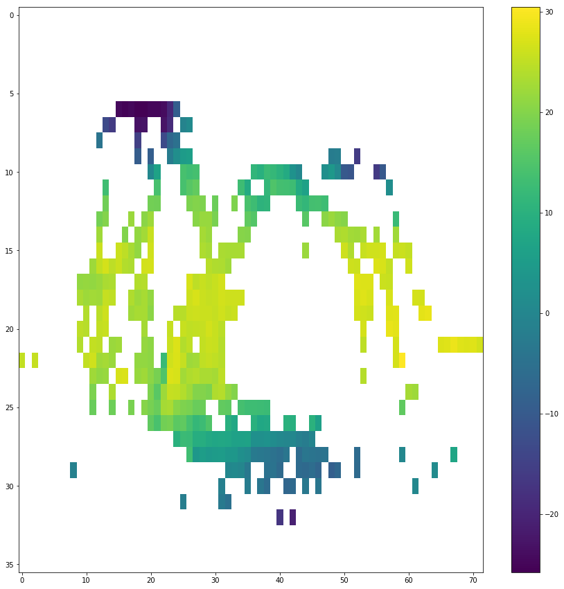
imshow askes for a special argument if you want to modify the aspect ratio.
f, ax = plt.subplots(1, 1, figsize=(15, 15))
c = ax.imshow(T1850, aspect='auto')
plt.colorbar(c)
<matplotlib.colorbar.Colorbar at 0x112cad470>
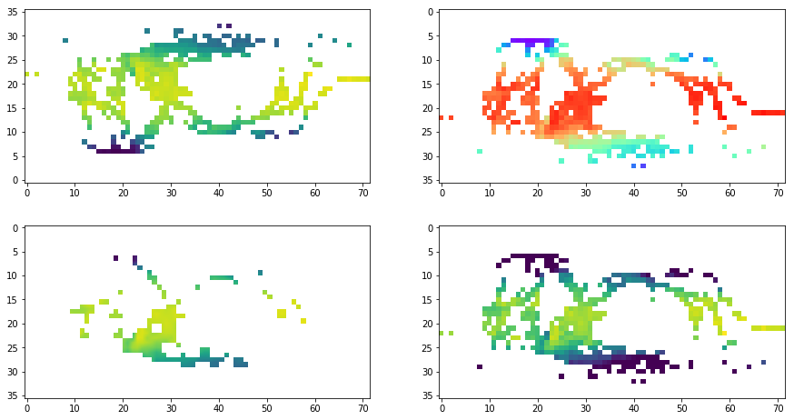
You can twick the figure with different colormap, origin, interpolation, vmin and vmax.
f, ax = plt.subplots(2, 2, figsize=(15, 8))
ax[0,0].imshow(T1850, origin='lower')
ax[0,1].imshow(T1850, cmap='rainbow')    # more at https://matplotlib.org/examples/color/colormaps_reference.html
ax[1,0].imshow(T1850, interpolation='bilinear')
ax[1,1].imshow(T1850, vmin=0, vmax=30)
<matplotlib.image.AxesImage at 0x11ba4fd30>
pcolormesh
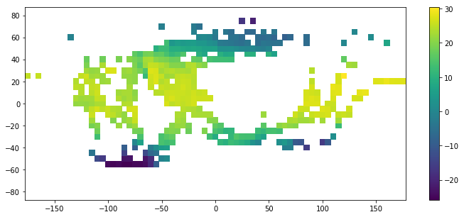
You can use pcolormesh in the same manner as imshow, but you can also pass the grid information.
help(plt.pcolormesh)
Help on function pcolormesh in module matplotlib.pyplot:

pcolormesh(*args, alpha=None, norm=None, cmap=None, vmin=None, vmax=None, shading='flat', antialiased=False, data=None, **kwargs)
    Create a pseudocolor plot with a non-regular rectangular grid.

    Call signature::

        pcolor([X, Y,] C, **kwargs)

    *X* and *Y* can be used to specify the corners of the quadrilaterals.

    .. note::

       ``pcolormesh()`` is similar to :func:`~Axes.pcolor`. It's much
       faster and preferred in most cases. For a detailed discussion on
       the differences see
       :ref:`Differences between pcolor() and pcolormesh()
       <differences-pcolor-pcolormesh>`.

    Parameters
    ----------
    C : array_like
        A scalar 2-D array. The values will be color-mapped.

    X, Y : array_like, optional
        The coordinates of the quadrilateral corners. The quadrilateral
        for ``C[i,j]`` has corners at::

            (X[i+1, j], Y[i+1, j])          (X[i+1, j+1], Y[i+1, j+1])
                                  +--------+
                                  | C[i,j] |
                                  +--------+
                (X[i, j], Y[i, j])          (X[i, j+1], Y[i, j+1]),

        Note that the column index corresponds to the
        x-coordinate, and the row index corresponds to y. For
        details, see the :ref:`Notes <axes-pcolormesh-grid-orientation>`
        section below.

        The dimensions of *X* and *Y* should be one greater than those of
        *C*. Alternatively, *X*, *Y* and *C* may have equal dimensions, in
        which case the last row and column of *C* will be ignored.

        If *X* and/or *Y* are 1-D arrays or column vectors they will be
        expanded as needed into the appropriate 2-D arrays, making a
        rectangular grid.

    cmap : str or `~matplotlib.colors.Colormap`, optional
        A Colormap instance or registered colormap name. The colormap
        maps the *C* values to colors. Defaults to :rc:`image.cmap`.

    norm : `~matplotlib.colors.Normalize`, optional
        The Normalize instance scales the data values to the canonical
        colormap range [0, 1] for mapping to colors. By default, the data
        range is mapped to the colorbar range using linear scaling.

    vmin, vmax : scalar, optional, default: None
        The colorbar range. If *None*, suitable min/max values are
        automatically chosen by the `~.Normalize` instance (defaults to
        the respective min/max values of *C* in case of the default linear
        scaling).

    edgecolors : {'none', None, 'face', color, color sequence}, optional
        The color of the edges. Defaults to 'none'. Possible values:

        - 'none' or '': No edge.
        - *None*: :rc:`patch.edgecolor` will be used. Note that currently
          :rc:`patch.force_edgecolor` has to be True for this to work.
        - 'face': Use the adjacent face color.
        - An mpl color or sequence of colors will set the edge color.

        The singular form *edgecolor* works as an alias.

    alpha : scalar, optional, default: None
        The alpha blending value, between 0 (transparent) and 1 (opaque).

    shading : {'flat', 'gouraud'}, optional
        The fill style, Possible values:

        - 'flat': A solid color is used for each quad. The color of the
          quad (i, j), (i+1, j), (i, j+1), (i+1, j+1) is given by
          ``C[i,j]``.
        - 'gouraud': Each quad will be Gouraud shaded: The color of the
          corners (i', j') are given by ``C[i',j']``. The color values of
          the area in between is interpolated from the corner values.
          When Gouraud shading is used, *edgecolors* is ignored.

    snap : bool, optional, default: False
        Whether to snap the mesh to pixel boundaries.

    Returns
    -------
    mesh : `matplotlib.collections.QuadMesh`

    Other Parameters
    ----------------
    **kwargs
        Additionally, the following arguments are allowed. They are passed
        along to the `~matplotlib.collections.QuadMesh` constructor:

      agg_filter: a filter function, which takes a (m, n, 3) float array and a dpi value, and returns a (m, n, 3) array
      alpha: float or None
      animated: bool
      antialiased: bool or sequence of bools
      array: ndarray
      capstyle: {'butt', 'round', 'projecting'}
      clim: a length 2 sequence of floats; may be overridden in methods that have ``vmin`` and ``vmax`` kwargs.
      clip_box: `.Bbox`
      clip_on: bool
      clip_path: [(`~matplotlib.path.Path`, `.Transform`) | `.Patch` | None]
      cmap: colormap or registered colormap name
      color: matplotlib color arg or sequence of rgba tuples
      contains: callable
      edgecolor: color or sequence of colors
      facecolor: color or sequence of colors
      figure: `.Figure`
      gid: str
      hatch: {'/', '\\', '|', '-', '+', 'x', 'o', 'O', '.', '*'}
      in_layout: bool
      joinstyle: {'miter', 'round', 'bevel'}
      label: object
      linestyle: {'-', '--', '-.', ':', '', (offset, on-off-seq), ...}
      linewidth: float or sequence of floats
      norm: `.Normalize`
      offset_position: {'screen', 'data'}
      offsets: float or sequence of floats
      path_effects: `.AbstractPathEffect`
      picker: None or bool or float or callable
      pickradius: unknown
      rasterized: bool or None
      sketch_params: (scale: float, length: float, randomness: float)
      snap: bool or None
      transform: `.Transform`
      url: str
      urls: List[str] or None
      visible: bool
      zorder: float


    See Also
    --------
    pcolor : An alternative implementation with slightly different
        features. For a detailed discussion on the differences see
        :ref:`Differences between pcolor() and pcolormesh()
        <differences-pcolor-pcolormesh>`.
    imshow : If *X* and *Y* are each equidistant, `~.Axes.imshow` can be a
        faster alternative.

    Notes
    -----

    **Masked arrays**

    *C* may be a masked array. If ``C[i, j]`` is masked, the corresponding
    quadrilateral will be transparent. Masking of *X* and *Y* is not
    supported. Use `~.Axes.pcolor` if you need this functionality.

    .. _axes-pcolormesh-grid-orientation:

    **Grid orientation**

    The grid orientation follows the standard matrix convention: An array
    *C* with shape (nrows, ncolumns) is plotted with the column number as
    *X* and the row number as *Y*.

    .. _differences-pcolor-pcolormesh:

    **Differences between pcolor() and pcolormesh()**

    Both methods are used to create a pseudocolor plot of a 2-D array
    using quadrilaterals.

    The main difference lies in the created object and internal data
    handling:
    While `~.Axes.pcolor` returns a `.PolyCollection`, `~.Axes.pcolormesh`
    returns a `.QuadMesh`. The latter is more specialized for the given
    purpose and thus is faster. It should almost always be preferred.

    There is also a slight difference in the handling of masked arrays.
    Both `~.Axes.pcolor` and `~.Axes.pcolormesh` support masked arrays
    for *C*. However, only `~.Axes.pcolor` supports masked arrays for *X*
    and *Y*. The reason lies in the internal handling of the masked values.
    `~.Axes.pcolor` leaves out the respective polygons from the
    PolyCollection. `~.Axes.pcolormesh` sets the facecolor of the masked
    elements to transparent. You can see the difference when using
    edgecolors. While all edges are drawn irrespective of masking in a
    QuadMesh, the edge between two adjacent masked quadrilaterals in
    `~.Axes.pcolor` is not drawn as the corresponding polygons do not
    exist in the PolyCollection.

    Another difference is the support of Gouraud shading in
    `~.Axes.pcolormesh`, which is not available with `~.Axes.pcolor`.

    .. note::
        In addition to the above described arguments, this function can take a
        **data** keyword argument. If such a **data** argument is given, the
        following arguments are replaced by **data[<arg>]**:

        * All positional and all keyword arguments.

        Objects passed as **data** must support item access (``data[<arg>]``) and
        membership test (``<arg> in data``).
# Use pcolormesh as imshow
f, ax = plt.subplots(1, 1, figsize=(12, 5))
c = ax.pcolormesh(T1850)
plt.colorbar(c)
<matplotlib.colorbar.Colorbar at 0x11fb12630>
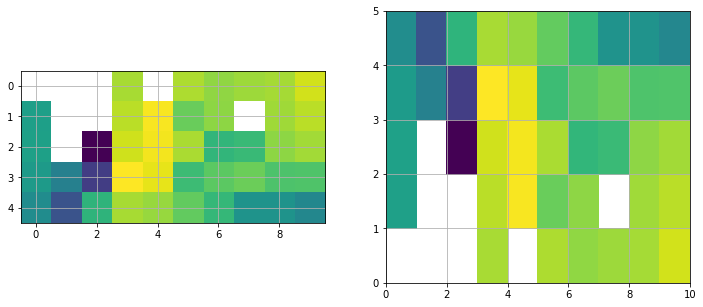
f, ax = plt.subplots(1, 2, figsize=(12, 5))
ax[0].imshow(T1850[20:25, 20:30])
ax[0].grid('on')

ax[1].pcolormesh(T1850[20:25, 20:30])
ax[1].grid('on')
/Users/hajsong/miniconda2/envs/py36/lib/python3.6/site-packages/matplotlib/cbook/__init__.py:424: MatplotlibDeprecationWarning:
Passing one of 'on', 'true', 'off', 'false' as a boolean is deprecated; use an actual boolean (True/False) instead.
  warn_deprecated("2.2", "Passing one of 'on', 'true', 'off', 'false' as a "
f, ax = plt.subplots(1, 1, figsize=(12, 5))
c = ax.pcolormesh(lon, lat, T1850)
plt.colorbar(c)
<matplotlib.colorbar.Colorbar at 0x115b63c88>
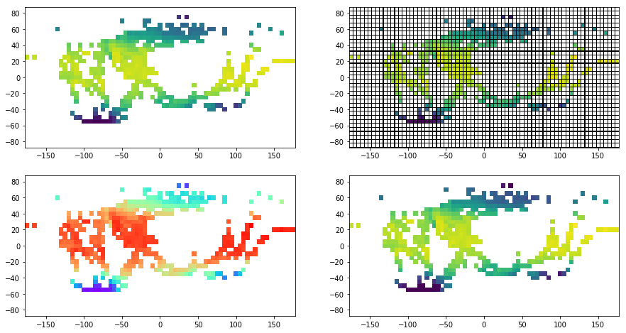
f, ax = plt.subplots(2, 2, figsize=(15, 8))
# pcolor() can be very slow for large arrays.
# In most cases you should use the similar but much faster pcolormesh instead
ax[0,0].pcolor(lon, lat, T1850)
ax[0,1].pcolormesh(lon, lat, T1850, edgecolors='black', linewidth=.1)
ax[1,0].pcolormesh(lon, lat, T1850, cmap='rainbow')    # more at https://matplotlib.org/examples/color/colormaps_reference.html
ax[1,1].pcolormesh(lon, lat, T1850, vmin=-20, vmax=30)
<matplotlib.collections.QuadMesh at 0x115841ac8>
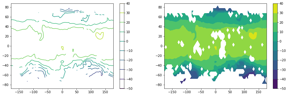
contour / contourf
contour and contourf draw contour lines and filled contours, respectively.
You can pass the grid information to these functions.
T2018 = T[0, :, :] + Tanom[2016, :, :] # monthly mean T for 2018 January
f, ax = plt.subplots(1, 2, figsize=(16, 5))
c0 = ax[0].contour(lon, lat, T2018)
plt.colorbar(c0, ax=ax[0])
c1 = ax[1].contourf(lon, lat, T2018)
plt.colorbar(c1, ax=ax[1])
<matplotlib.colorbar.Colorbar at 0x115e1b438>
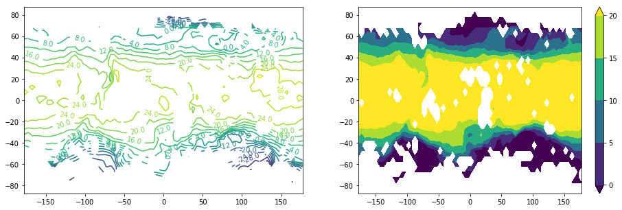
You can decide how many contours to show in two different ways: a number of contours or an actual range
f, ax = plt.subplots(1, 2, figsize=(16, 5))
c0 = ax[0].contour(lon, lat, T2018, 20)
ax[0].clabel(c0, inline=1, fontsize=10, fmt='%2.1f')
c1 = ax[1].contourf(lon, lat, T2018, np.arange(0, 21, 5), extend='both')
# ax[1].clabel(c1)
plt.colorbar(c1, ax=ax[1])
<matplotlib.colorbar.Colorbar at 0x119b52ac8>
Quiver
This is useful when you want to show the wind or ocean current.
Let’s read the wind data.
f = Dataset('uwnd.mon.mean.nc', 'r')
print(f.variables.keys())
uwind = f.variables['uwnd'][:]    # monthly data
lon = f.variables['lon'][:]
lat = f.variables['lat'][:]
f.close()
f = Dataset('vwnd.mon.mean.nc', 'r')
print(f.variables.keys())
vwind = f.variables['vwnd'][:]    # monthly data
lon = f.variables['lon'][:]
lat = f.variables['lat'][:]
f.close()
odict_keys(['lat', 'lon', 'time', 'uwnd'])
odict_keys(['lat', 'lon', 'time', 'vwnd'])
help(plt.quiver)
Help on function quiver in module matplotlib.pyplot:

quiver(*args, data=None, **kw)
    Plot a 2-D field of arrows.

    Call signatures::

      quiver(U, V, **kw)
      quiver(U, V, C, **kw)
      quiver(X, Y, U, V, **kw)
      quiver(X, Y, U, V, C, **kw)

    *U* and *V* are the arrow data, *X* and *Y* set the location of the
    arrows, and *C* sets the color of the arrows. These arguments may be 1-D or
    2-D arrays or sequences.

    If *X* and *Y* are absent, they will be generated as a uniform grid.
    If *U* and *V* are 2-D arrays and *X* and *Y* are 1-D, and if ``len(X)`` and
    ``len(Y)`` match the column and row dimensions of *U*, then *X* and *Y* will be
    expanded with :func:`numpy.meshgrid`.

    The default settings auto-scales the length of the arrows to a reasonable size.
    To change this behavior see the *scale* and *scale_units* kwargs.

    The defaults give a slightly swept-back arrow; to make the head a
    triangle, make *headaxislength* the same as *headlength*. To make the
    arrow more pointed, reduce *headwidth* or increase *headlength* and
    *headaxislength*. To make the head smaller relative to the shaft,
    scale down all the head parameters. You will probably do best to leave
    minshaft alone.

    *linewidths* and *edgecolors* can be used to customize the arrow
    outlines.

    Parameters
    ----------
    X : 1D or 2D array, sequence, optional
        The x coordinates of the arrow locations
    Y : 1D or 2D array, sequence, optional
        The y coordinates of the arrow locations
    U : 1D or 2D array or masked array, sequence
        The x components of the arrow vectors
    V : 1D or 2D array or masked array, sequence
        The y components of the arrow vectors
    C : 1D or 2D array, sequence, optional
        The arrow colors
    units : [ 'width' | 'height' | 'dots' | 'inches' | 'x' | 'y' | 'xy' ]
        The arrow dimensions (except for *length*) are measured in multiples of
        this unit.

        'width' or 'height': the width or height of the axis

        'dots' or 'inches': pixels or inches, based on the figure dpi

        'x', 'y', or 'xy': respectively *X*, *Y*, or :math:`\sqrt{X^2 + Y^2}`
        in data units

        The arrows scale differently depending on the units.  For
        'x' or 'y', the arrows get larger as one zooms in; for other
        units, the arrow size is independent of the zoom state.  For
        'width or 'height', the arrow size increases with the width and
        height of the axes, respectively, when the window is resized;
        for 'dots' or 'inches', resizing does not change the arrows.
    angles : [ 'uv' | 'xy' ], array, optional
        Method for determining the angle of the arrows. Default is 'uv'.

        'uv': the arrow axis aspect ratio is 1 so that
        if *U*==*V* the orientation of the arrow on the plot is 45 degrees
        counter-clockwise from the horizontal axis (positive to the right).

        'xy': arrows point from (x,y) to (x+u, y+v).
        Use this for plotting a gradient field, for example.

        Alternatively, arbitrary angles may be specified as an array
        of values in degrees, counter-clockwise from the horizontal axis.

        Note: inverting a data axis will correspondingly invert the
        arrows only with ``angles='xy'``.
    scale : None, float, optional
        Number of data units per arrow length unit, e.g., m/s per plot width; a
        smaller scale parameter makes the arrow longer. Default is *None*.

        If *None*, a simple autoscaling algorithm is used, based on the average
        vector length and the number of vectors. The arrow length unit is given by
        the *scale_units* parameter
    scale_units : [ 'width' | 'height' | 'dots' | 'inches' | 'x' | 'y' | 'xy' ], None, optional
        If the *scale* kwarg is *None*, the arrow length unit. Default is *None*.

        e.g. *scale_units* is 'inches', *scale* is 2.0, and
        ``(u,v) = (1,0)``, then the vector will be 0.5 inches long.

        If *scale_units* is 'width'/'height', then the vector will be half the
        width/height of the axes.

        If *scale_units* is 'x' then the vector will be 0.5 x-axis
        units. To plot vectors in the x-y plane, with u and v having
        the same units as x and y, use
        ``angles='xy', scale_units='xy', scale=1``.
    width : scalar, optional
        Shaft width in arrow units; default depends on choice of units,
        above, and number of vectors; a typical starting value is about
        0.005 times the width of the plot.
    headwidth : scalar, optional
        Head width as multiple of shaft width, default is 3
    headlength : scalar, optional
        Head length as multiple of shaft width, default is 5
    headaxislength : scalar, optional
        Head length at shaft intersection, default is 4.5
    minshaft : scalar, optional
        Length below which arrow scales, in units of head length. Do not
        set this to less than 1, or small arrows will look terrible!
        Default is 1
    minlength : scalar, optional
        Minimum length as a multiple of shaft width; if an arrow length
        is less than this, plot a dot (hexagon) of this diameter instead.
        Default is 1.
    pivot : [ 'tail' | 'mid' | 'middle' | 'tip' ], optional
        The part of the arrow that is at the grid point; the arrow rotates
        about this point, hence the name *pivot*.
    color : [ color | color sequence ], optional
        This is a synonym for the
        :class:`~matplotlib.collections.PolyCollection` facecolor kwarg.
        If *C* has been set, *color* has no effect.

    Notes
    -----
    Additional :class:`~matplotlib.collections.PolyCollection`
    keyword arguments:

      agg_filter: a filter function, which takes a (m, n, 3) float array and a dpi value, and returns a (m, n, 3) array
      alpha: float or None
      animated: bool
      antialiased: bool or sequence of bools
      array: ndarray
      capstyle: {'butt', 'round', 'projecting'}
      clim: a length 2 sequence of floats; may be overridden in methods that have ``vmin`` and ``vmax`` kwargs.
      clip_box: `.Bbox`
      clip_on: bool
      clip_path: [(`~matplotlib.path.Path`, `.Transform`) | `.Patch` | None]
      cmap: colormap or registered colormap name
      color: matplotlib color arg or sequence of rgba tuples
      contains: callable
      edgecolor: color or sequence of colors
      facecolor: color or sequence of colors
      figure: `.Figure`
      gid: str
      hatch: {'/', '\\', '|', '-', '+', 'x', 'o', 'O', '.', '*'}
      in_layout: bool
      joinstyle: {'miter', 'round', 'bevel'}
      label: object
      linestyle: {'-', '--', '-.', ':', '', (offset, on-off-seq), ...}
      linewidth: float or sequence of floats
      norm: `.Normalize`
      offset_position: {'screen', 'data'}
      offsets: float or sequence of floats
      path_effects: `.AbstractPathEffect`
      picker: None or bool or float or callable
      pickradius: unknown
      rasterized: bool or None
      sketch_params: (scale: float, length: float, randomness: float)
      snap: bool or None
      transform: `.Transform`
      url: str
      urls: List[str] or None
      visible: bool
      zorder: float

    See Also
    --------
    quiverkey : Add a key to a quiver plot
f, ax = plt.subplots(1, 1, figsize=(16, 8))
q = ax.quiver(lon, lat, uwind[-1, :, :], vwind[-1, :, :])
# q = ax.quiver(lon, lat, uwind[-1,...], vwind[-1,...])
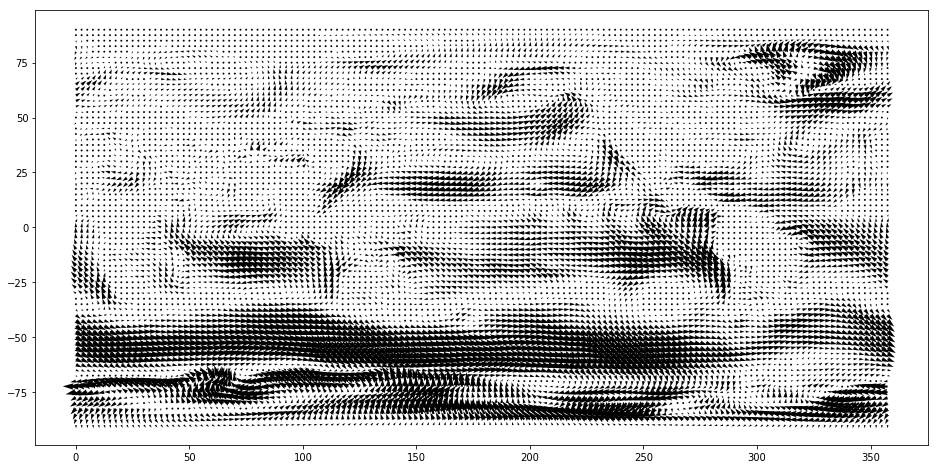
Although we have the plot with arrows, it is not easy to see their sizes and direction.
It seems that there needs some tunings.
help(plt.quiverkey)
Help on function quiverkey in module matplotlib.pyplot:

quiverkey(Q, X, Y, U, label, **kw)
    Add a key to a quiver plot.

    Call signature::

      quiverkey(Q, X, Y, U, label, **kw)

    Arguments:

      *Q*:
        The Quiver instance returned by a call to quiver.

      *X*, *Y*:
        The location of the key; additional explanation follows.

      *U*:
        The length of the key

      *label*:
        A string with the length and units of the key

    Keyword arguments:

      *angle* = 0
        The angle of the key arrow. Measured in degrees anti-clockwise from the
        x-axis.

      *coordinates* = [ 'axes' | 'figure' | 'data' | 'inches' ]
        Coordinate system and units for *X*, *Y*: 'axes' and 'figure' are
        normalized coordinate systems with 0,0 in the lower left and 1,1
        in the upper right; 'data' are the axes data coordinates (used for
        the locations of the vectors in the quiver plot itself); 'inches'
        is position in the figure in inches, with 0,0 at the lower left
        corner.

      *color*:
        overrides face and edge colors from *Q*.

      *labelpos* = [ 'N' | 'S' | 'E' | 'W' ]
        Position the label above, below, to the right, to the left of the
        arrow, respectively.

      *labelsep*:
        Distance in inches between the arrow and the label.  Default is
        0.1

      *labelcolor*:
        defaults to default :class:`~matplotlib.text.Text` color.

      *fontproperties*:
        A dictionary with keyword arguments accepted by the
        :class:`~matplotlib.font_manager.FontProperties` initializer:
        *family*, *style*, *variant*, *size*, *weight*

    Any additional keyword arguments are used to override vector
    properties taken from *Q*.

    The positioning of the key depends on *X*, *Y*, *coordinates*, and
    *labelpos*.  If *labelpos* is 'N' or 'S', *X*, *Y* give the position
    of the middle of the key arrow.  If *labelpos* is 'E', *X*, *Y*
    positions the head, and if *labelpos* is 'W', *X*, *Y* positions the
    tail; in either of these two cases, *X*, *Y* is somewhere in the
    middle of the arrow+label key object.
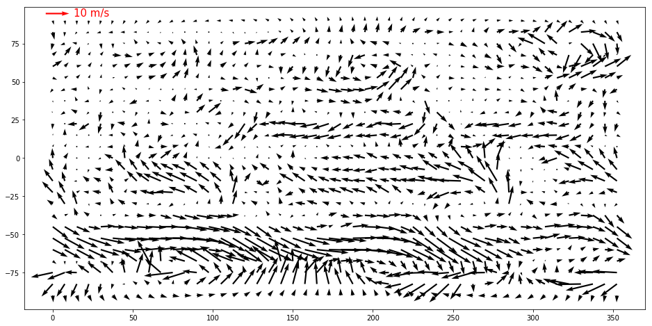
f, ax = plt.subplots(1, 1, figsize=(16, 8))
# Try to show arrows at every three points.
intv = 3
q = ax.quiver(lon[::intv], lat[::intv], uwind[-1, ::intv, ::intv], vwind[-1, ::intv, ::intv])
qk = ax.quiverkey(q, 10, 95, 10, '10 m/s', labelpos='E', coordinates='data',
                  color='r', labelcolor='r', fontproperties={'size': 15})
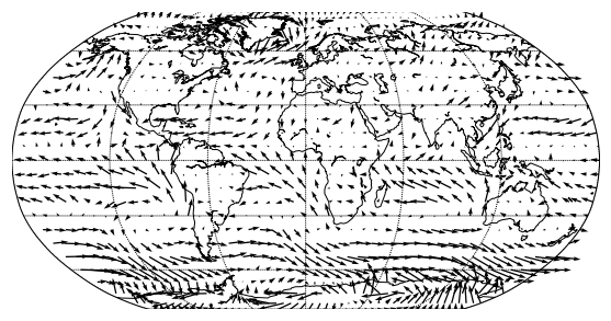
from mpl_toolkits.basemap import Basemap

X, Y =np.meshgrid(lon, lat)
plt.figure(figsize=(15,5))
m = Basemap(projection='robin',lon_0=0,resolution='c')
m.drawcoastlines()
m.drawparallels(np.arange(-90.,120.,30.))
m.drawmeridians(np.arange(0.,360.,60.))
m.quiver(X[::intv, ::intv], Y[::intv, ::intv], uwind[-1, ::intv, ::intv], vwind[-1, ::intv, ::intv], latlon=True)