Statistical analysis
- Confidence intervals
- Linear Regression
- Correlation
This lecture is based on the Chapter 3 in Data analysis methods in Physical Oceanography by Thomson and Emery.
Sample distribution
Fundamental to any form of data analysis is the realization that we are usually working with a limited set (or sample) of random events drawn from a much larger population. To describe the sample, we often use the concept of the sample mean. If the sample has $N$ data values, $x_1, x_2, \cdots, x_N$, the sample mean can be expressed as
$$ \bar{x} = \frac{1}{N} \sum^N_{i=1} x_i. $$
The sample mean is an unbiased estimate of the true population mean, $\mu$. An “unbiased” estimator means that it is equal to the expected value, $E[x]$ so that $E[x] = \mu$. We will come back to this concept later.
The sample mean locates the center of mass of the data distribution such that
$$ \sum^N_{i=1}(x_i - \bar{x}) = 0, $$
that is, the sample mean splits the data so that there is an equal weighting of negative and positive values.
You may give weight, $f_i$, on each sample. Then the weighted sample mean is defined as
$$ \bar{x} = \frac{1}{N} \sum^N_{i=1} f_i x_i. $$
It is clear that the sample mean is recovered with the weights all equal to 1 in the weighted sample mean.
The sample mean values give us the center of mass of a data distribution. How about the spread of the data? To determine it, we need a measure of the sample variability or sample standard deviation, $s’$, which is expressed in terms of the positive square root of the sample variance, the average of the square of the sample deviation.
$$ s’^2 = \frac{1}{N} \sum^N_{i=1} (x_i - \bar{x})^2. $$
This measure expresses the typical difference of a data value from the mean value of all the data points. In general, it differs from the true population variance, $\sigma^2$, and the population standard deviation, $\sigma$, indicating that $s’$ is biased. An unbiased estimator of the population variance, $s$, is obtained from
$$ s^2 = \frac{1}{(N-1)} \sum^N_{i=1} (x_i - \bar{x})^2. $$
Again, we will come back to this concept later.
The difference between the sample standard deviation and population standard deviation becomes significant when the sample size is small ($N<30$).
Other statistical values of importance are the range, mode, and median of a data distribution. The range is another measure for the spread and represents the difference between two extreme points. The mode is the value that occurs the most, while the median is the value at the middle of the distribution.
Moments and expected values
To describe the distribution and the related probability, we often compute parameters called “moments”. The first two moments are already introduced: the population mean and standard deviation. In general, these two moments are not enough to completely describe the distribution, except the normal (Gaussian) distribution.
When discussing moments, it is useful to introduce the concept of expected values. This concept is analogous to the notion of weighted functions. If we know the probability function, $P(x)$, for the event $x$, the expected value for a discrete PDF is
$$ E[X] = \sum^N_{i=1} x_iP(x_i) = \mu, $$
where $\mu$ is the population mean introduced earlier. As you can notice, this has very similar form to the weighted average. The difference is that the weighted average consider a single set of experimental samples whereas $P(x)$ is the expected relative frequency for an infinite number of samples from repeated trials of the experiment.
The variance of the random variable $X$ is the expected value of $(X-\mu)^2$, or
$$ V[X] = E[(X-\mu)^2] = \sum^N_{i=1}(x_i-\mu)^2P(x_i) = \sigma^2. $$
Here are some properties of expected values for random variables:
- For $c=constant$, $E[c] = c, V[c] = 0$.
- $E[cg(X)] = cE[g(X)], V[cg(X)] = c^2V[g(X)]$
- $E[g_1(X) \pm g_x(X) \pm \dots] = E[g_1(X)] \pm E[g_1(X)] \pm \dots$
- $V[g(X)] = E[(g(X) - \mu)^2] = E[g(X)^2]-\mu^2$
- $E[g_1g_2] = E[g_1]E[g_2]$
- $V[g_1\pm g_2] = V[g_1] + V{g_2} \pm 2C[g_1, g_2]$ (where $C[g_1,g_2] = E[g_1g_2] - E[g_1]E[g_2]$)
The covariance function, $C[g_1, g_2]$ is zero when $g_1$ and $g_2$ are independent random variables.
Using the properties above, we can get the first and second moments of $Y = a + bX$ as
$$ E[Y] = E[a+bX] = a+bE[x] $$
and
$$ V[Y] = V[a+bX] = b^2V[x]. $$
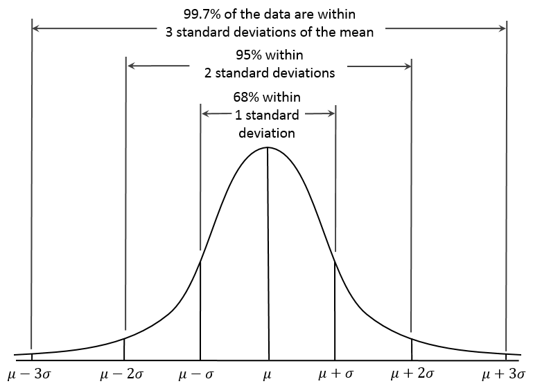
The normal distribution
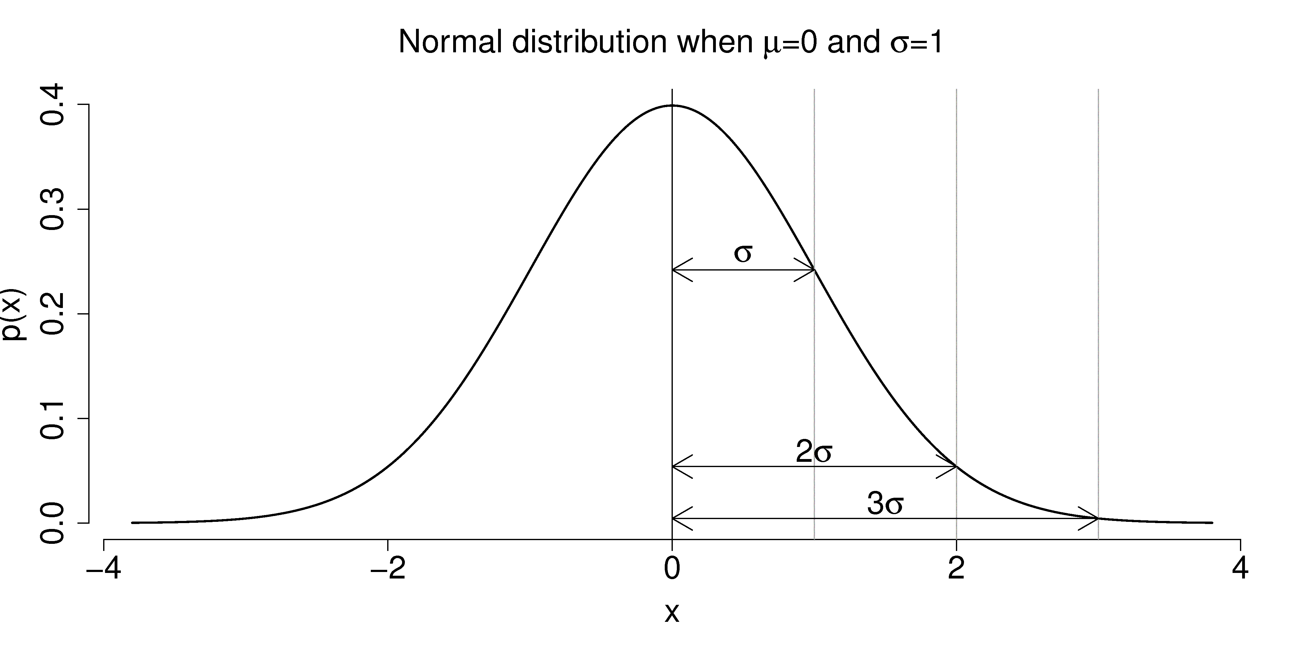
Perhaps the most familiar and widely used probability density function is the normal (Gaussian) density function:
The standardized normal variable, $Z$ for the normal distribution gives the distance of points measured from the mean of the normal random variable in terms of the standard deviation of the normal random variable, $X$.
$$
f(x) = \frac{1}{\sqrt{2\pi\sigma^2}}exp\left(-\frac{(x-\mu)^2}{2\sigma^2}\right)
$$
The probability between in the interval $a$ and $b$ is given by the integral of $f(x)$.
$$ P(a \le X \le b) = \int^b_a \frac{1}{\sqrt{2\pi\sigma^2}}exp\left(-\frac{(x-\mu)^2}{2\sigma^2}\right)dx $$
For normal distribution, we can come up with the distribution for the normalized variable, $Z$,
$$ Z = \frac{X-\mu}{\sum} $$
This is called the standardized normal variable. It gives the distance of points measured from the mean of the normal random variable in terms of the standard deviation of the normal random variable, $X$.
Central limit theorem
Please see the link, and jupyter notebook.